Parallel Random Forest
Kirn Hans (khans) and Sally McNichols (smcnicho)
Summary
We used CUDA to implement the decision tree learning algorithm specified in the CUDT paper on the GHC cluster machines. Our deliverable is parallel code for training decision trees written in CUDA and a comparison against decision tree code written in sklearn for Python and randomForest for R.
Background
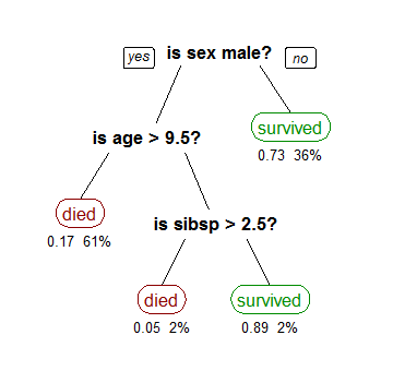
Decision trees are a common classification method in statistics/machine learning. It takes as an input a training set and a testing set. A decision tree divides the training dataset based on the values of the attribute, e.g. age in the figure shown. Each node is divided into children based on a attribute’s value, e.g. age’s value of 9.5. The value is chosen to divide the dataset to maximize the separation of different classifications, e.g the separation of died and survived. This is called splitting a node.
Source: https://en.wikipedia.org/wiki/Decision_tree_learning
When we are training a tree, we have to determine the attributes and values on which to split nodes. Any attribute can be chosen and any potential value for the attribute can be chosen. To split a node, we calculate the Gini impurity from the resulting dataset, a measure that indicates the degree of variation. We want to minimize the Gini impurity. The options to calculate over are for each attribute, each value of the attribute, and all the datapoints in the training set for the attribute.
After splitting the node, we split its children and repeat the process until we have very low impurity. The calculations are independent for each subtree. Calculating impurity is also independent for each attribute for a given node. Each level however, is completely dependent on the previous level. This calculation is data parallel and probably amenable to SIMD execution. There is little locality because of the independence of the subset for each tree and the randomness of the rows of a single subset.
Approach
We used CUDA to run our code on GPUs. Specifically, we implemented the decision tree training algorithm defined in the CUDT paper. This required implementing 3 main algorithms in CUDA: build attribute lists, find split points, and split attribute lists.
Here is a breakdown of the tasks assigned to the CPU and GPU.

Source: https://www.hindawi.com/journals/tswj/2014/745640/fig2/
From this diagram, we see that actually constructing the decision tree and performing classification is performed on the CPU. We specifically use the GPU for the heavy computation tasks like building the attribute lists, finding the best split point for a node, and splitting the data based on the best split point.
On the CPU side, we implemented a standard sequential CART algorithm. We used the gini index as the split criterion, and we did not limit the tree depth. The general algorithm does as follows:
Grow(tree):
- For all the data in this node, find the best split point (make call to device code)
- Generate a left child and right child by splitting the data at split point (make call to device code)
- If left child is not terminal, grow the left child
- If right child is not terminal, grow the right child
The result of this algorithm is a DecisionTree C++ object that can be evaluated on the CPU for performing classification.
Now we discuss the GPU code that aids building the decision tree. The CUDT algorithm is built off of SPRINT, which is another algorithm for building parallel decision trees. The main idea behind SPRINT is to transform the training data into a set of attribute lists. An attribute list is created for each attribute/variable in the dataset, and it is composed of 3 things: a list of the data values for the attribute, a list of the class labels for each data point, and a list of row ids that correspond to the data point.
Example: Here we have a data set that has 2 attributes: Age and Car type. Therefore, we split the dataset into 2 attribute lists. Each list has every value from the original dataset for that attribute, as well as the label and row number for that datapoint.

Source: https://www.hindawi.com/journals/tswj/2014/745640/fig2/
Another point to note is that each attribute list is sorted by the data value as a sort key. This will help calculate note splitting in parallel, as we will discuss later.
Storing the data in attribute lists is required for the CUDT algorithm because this allows us to process attributes in parallel, which in turn allows us to calculate the gini indexes of possible split points in parallel.
The algorithm for building the attribute lists is as follows:
- For each attribute A:
- Initialize arrays: values, labels, row_ids
- Launch kernel to populate values, labels, and row_ids
- Sort each of values, labels, and row_ids using values as the sort key
Note: For sorting, we use the thrust stable_sort_by_key function.
Once we have the data stored in attribute lists, we are able to calculate the best split point for the data. Because the data values in the attribute lists are sorted, we are able to consider splitting the data values list at a given index the same as splitting the node off that attribute. In order to calculate the Gini index of these possible splits, we use scan (parallel prefix-sum) on the list of class labels for counting the number of positive and negative data points that go into the left subtree. Specifically, index i of scan(class_labels) gives the number of positive data points that go into the left tree. This, along with the index number, size of the data array, and the final index of scan(class_labels) gives us enough information to calculate the Gini index for splitting on each value.
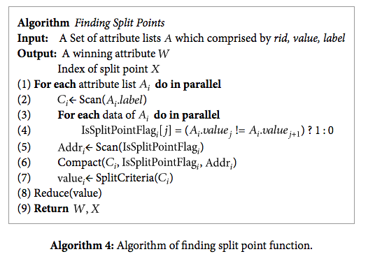
Source: https://www.hindawi.com/journals/tswj/2014/745640/alg4/
Note: We use thrust inclusive_scan for the scan operation and thrust min_element for the reduce operation.
In addition, we remove duplicate attribute values by performing a compact operation. Removing duplicates is important because we need to make sure that we don’t have repeat values going onto separate sides of the decision tree.
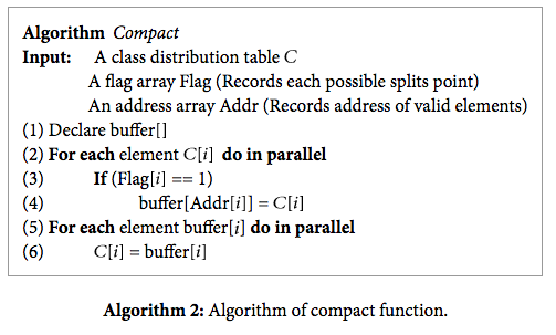
Source: https://www.hindawi.com/journals/tswj/2014/745640/alg2/
Once split points are computed, we need to actually split the attribute lists into the left subtree and right subtree. Because of the way that each attribute list is constructed, we can partition it so that the values that go in the left subtree are in the beginning of the array and the values that go into the right subtree are in the end of the array. This way we can just do some pointer arithmetic to point to the right subtree and left subtree data instead of having to copy the data or keep an extra list of indexes at each node.
The way that we partition each attribute list is first by finding the row indexes of values in the left subtree. We can get this information from the attribute list of the attribute that we are splitting on. Then we just use this to create a mask for partitioning each attribute list.
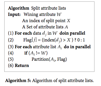
Source: https://www.hindawi.com/journals/tswj/2014/745640/alg5/
Note: We use thrust stable_partition to perform the partition operation.
Results
We measured speedup of our CUDA program against sklearn and python libraries. We ran our algorithm on three different pairs of training and testing datasets. The first set (cancer statistics) had a training set of 513 rows and a testing set of 172 rows, with 9 columns/attributes. The second set (loan statistics) had a training set of 656439 rows and a testing set of 221721 rows, with 13 columns/attributes. The third set (marketing statistics) had a training set of 33909 rows and testing set of 11304 rows, with 6 columns.
Our baseline was single-threaded CPU code. The libraries in python and sklearn are commonly used for machine learning purposes, so they are the de facto standard.
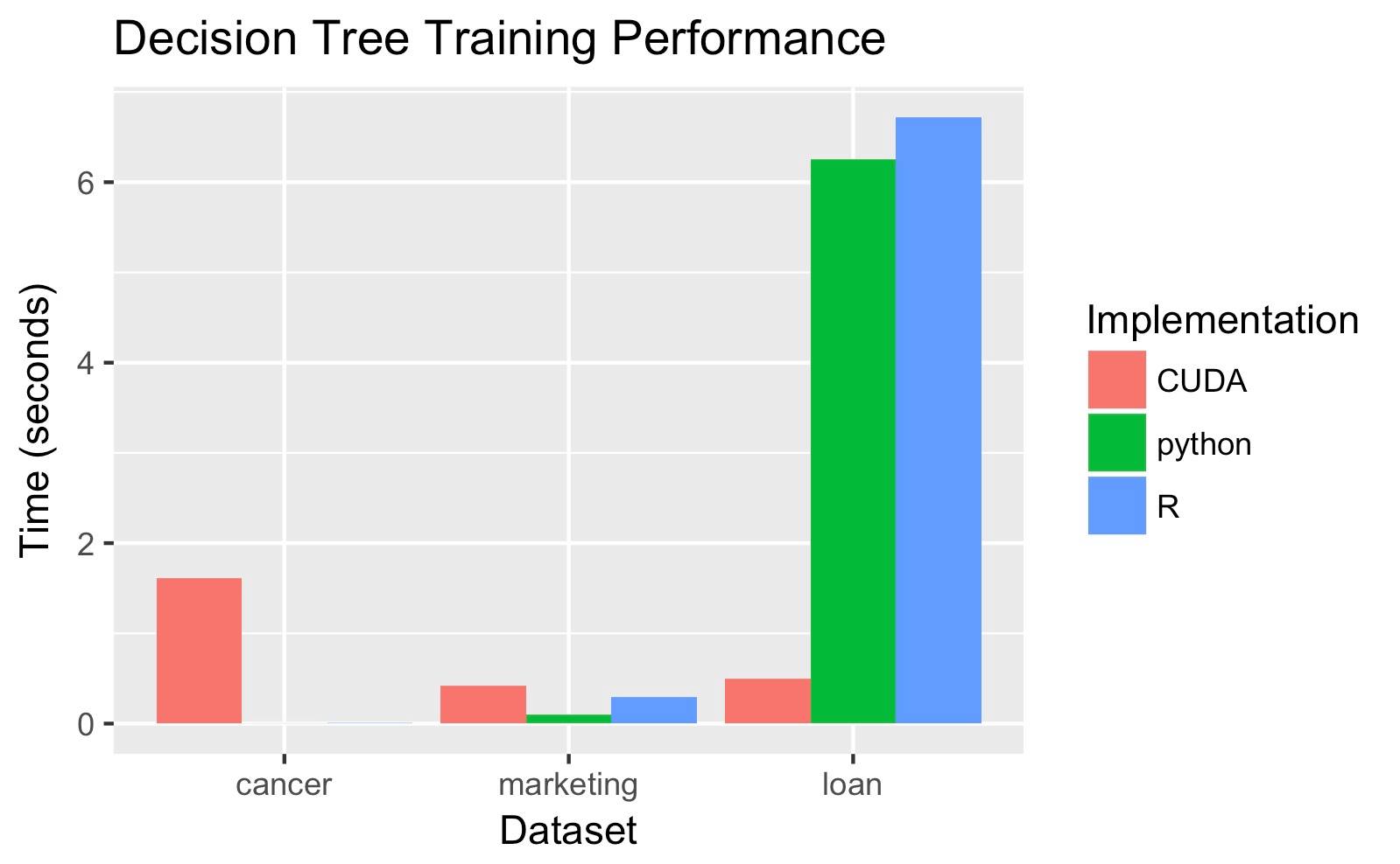
We generate different decision trees so our code is not entirely correct, and we are not convinced that our code is displaying accurate speedup for the second two datasets.
Our code is faster on larger datasets because once they have been copied over, they parallelize well and show the gains of GPU parallelism against the sequential CPU algorithms. Different datasets of the same size can affect workload because the impurity of the data set determines the time taken by training and testing. A dataset with more attributes is more likely to have more variation and thus more levels, so building the levels of the decision tree takes more time.
Our speedup is primarily limited by the overhead of copying data over to the GPUs. Every row in the dataset is likely to be in a subset used to train some tree and each GPU thread touches every tree, therefore, the entire dataset had to be copied over. For the smallest training set with 512 rows, it took 0.3 seconds just to copy over the data before training the trees, while the R implementation took 0.1 seconds to complete training overall.
Our speedup is also limited by the lack of parallelism in building multiple levels of a single tree. A very impure dataset requires a lot of levels and each level depends on the previous one. The splitting of a node depends on the subset of the data that falls in the range defined by its parent, so we can’t calculate a child node’s dataset’s impurity before the parent’s splitting. Deeper trees take significantly longer, as seen with our cancer dataset which had depth 38, vs. the other datasets that were shallower and had depth 2.
A CPU might have been a better choice because some parts of the program were amenable to SIMD execution. Having to copy the data over to each device added a large communication overhead. The calculations on the datasets suggest that the problem lent itself to a GPU though, given how GPUs are useful for matrix multiplication. A hybrid approach could lead to better results.
References
- CUDT: https://www.hindawi.com/journals/tswj/2014/745640/
- SPRINT: http://www.vldb.org/conf/1996/P544.PDF
- CSV parsing: https://github.com/ben-strasser/fast-cpp-csv-parser
- CUDA: 418 Homework 2 starter code
- Thrust: http://docs.nvidia.com/cuda/thrust/